Over on Bluesky, I’m following along as Loren Schmidt is working on their open world roguelike. Through her work, I learned about tabular lookup cellular automata.
It turns out to be one of those rare case where picking up a pebble on the beach reveals an entire mountain underneath.

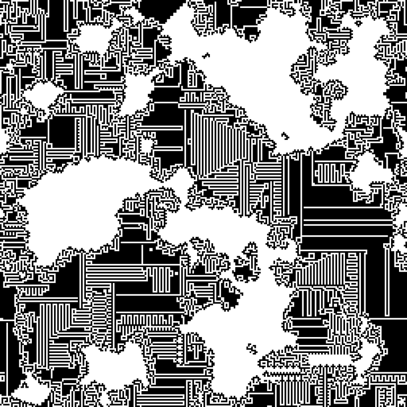
The idea is surprisingly simple. The starting state is a grid of cells, or pixels, either on or off, a regular pattern, random snow, Perlin noise, or anything we can think of. For each cell, the next state is determined by examining its state and that of its environment. A preset set of rules decides what happens with the cell. This can be done in 1D, 2D, 3D…
There’s good introductory material to be found on cellular automata , I recommend Daniel Shiffman’s Nature of Code https://natureofcode.com/cellular-automata/
What was new for me in Loren’s approach was twofold: the definition of the rules and how a rule is selected per cell.
1. In addition to the classical rules “switch on”, “switch off”, a third rule is introduced : “remain unchanged”.
2 . In her 2D explorations, the state of each cells is determined by two numbers, the number of active neighbors in the cardinal directions, up, down, left, right; and the number of active neighbors in the diagonal directions. Both numbers are in the range [0,4] and together they describe an entry in a 5×5 rule table. Each entry in the rule table is one of the three possible rules, “off”, “on”, “remain”. Note that in this case the state of the cell itself is not part of the rule selection.
A straightforward Processing implementation: can be found here. This system of CA can generate any number of evocative “environments”.


The parameter space is huge. Three possible rules in 25 table entries gives us 3^25 possibilities, 847.288.609.443. An impossible large number to exhaustingly catalogue and although the number of interesting seeds is equally large, they are rather sparse. So finding them is a matter of exploration and recording your findings. (Seriously, always record your seeds when doing generative art.)
In other to further explore this, for me, new type of CA, I took a step back and worked with a 1D variation, Processing sample downloadable here. Very much like the classical Wolfram CA, not plotting a 2D state but a time evolution of a 1D state, each line representing the next step.
The ruleset space I chose is again determined by 2 numbers, the number of active nearest neighbors; and the number of active next-nearest neighbors. Both numbers are in the range [0,2], and together give an entry in a 3×3 table. All in all, a more manageable 19.683 possibilities.


Because the parameter space is smaller and because it is more straightforward to autodetect repetition with 1D generations, I was able to chart the average number of cycles it takes for each ruleset to stabilize in a fixed cycle of repetition (depending on size and initial conditions). From that analysis I’ve added a list to the archive of the 3000+ rulesets that tend to generate the images with the least repetition, the longest cycle.