Disclaimer: there’s nothing wrong with using a sdf this way.
Recently, my good friend Mike Brondbjerg posted this on Twitter:
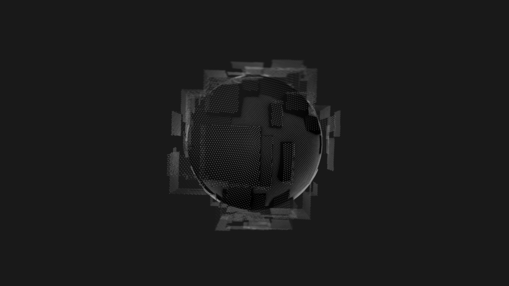
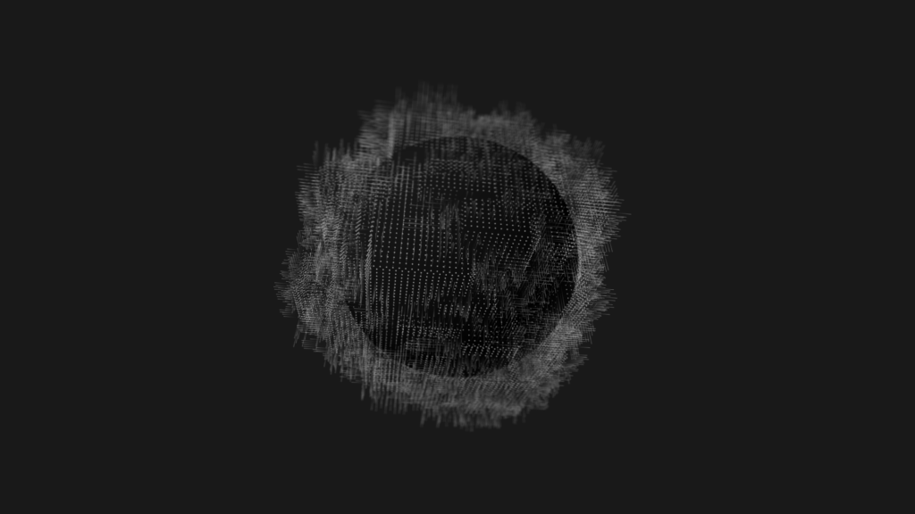
Dark Matter: 50,000 particles passing through a field until they hit a hidden sphere. By varying the distance travelled each step, the collisions are more / less accurate, so creating a nice fuzziness around the spheres. #generative #design #creativecommuting #creativecoding pic.twitter.com/gmFEV7fCwk
— Mike Brondbjerg (@mikebrondbjerg) January 15, 2020
You can follow along and see how this idea is evolving into the beautiful, elegant line drawings that are the hallmark of his style.
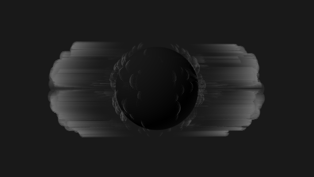
Dark Matter: random walk obstacle avoidance… nice random output. #creativecoding #generative #design #processing pic.twitter.com/DTzy7H2G6Z
— Mike Brondbjerg (@mikebrondbjerg) January 26, 2020
Spheres
Mike’s post gave me an idea, a way to introduce a concept I like to use in some of my work: signed distance functions. Sdfs are more commonly associated with raytracing and shaders, and by far the best source to learn about them in that context is Inigo Quilez, of Shadertoy fame: https://iquilezles.org/.
But there is a delightfully wrong way to use a sdf. Their primary use in raytracing and shaders is to define meshless geometry. For example, a way to draw smooth spheres without generating a ton of triangles. The use I’m showing here is the exact opposite: to generate geometry, point clouds in fact. Geometry that then needs to be processed in a conventional way before it can be rendered on the screen.
Let’s imagine we want to tackle something similar to the tweet: particles colliding with a sphere. One way to do this is by calculating the distance of the particle to the center of the sphere, let’s keep it at the origin. For a particle \vec{p} at position (x,y,z) , this distance is given by: {d( \vec{p} )=\sqrt{x.x+y.y+z.z}}. If that distance d is larger than the radius r of the sphere, the particle is outside the sphere, if it’s smaller then it is inside, if it’s exactly the same then it is on the surface.
\begin{cases} d( \vec{p} )<r, & \text{if } \vec{p}\text{ is inside} \\ d( \vec{p} )=r , & \text{if } \vec{p}\text{ is on sphere}\\ d( \vec{p} )>r, & \text{if } \vec{p}\text{ is outside} \end{cases}
Using this, we can check the particles every step. As long as their distance to the sphere is larger than the radius, they’re fine. If a particle takes a step and its distance becomes smaller or equal, it has hit the sphere.
If the sphere is not in the origin but centered in a point \vec{c} (cx,cy,cz) the distance function becomes {d( \vec{p} , \vec{c} )=\sqrt{(x-cx).(x-cx)+(y-cy).(y-cy)+(z-cz).(z-cz)}}. Typically, this is explained as the length of the vector going from \vec{p} to \vec{c} . Another way to see it, that will serve us well further on, is to imagine that we shift the sphere to the origin, \vec{c}\to\vec{0} , and the entire space moves with it . Our particle is then moved \vec{p}\to\vec{p}-\vec{c} . Checking a particle at \vec{p} against a sphere in center \vec{c} is the same as doing it for a particle at \vec{p}-\vec{c} against a sphere in the origin.
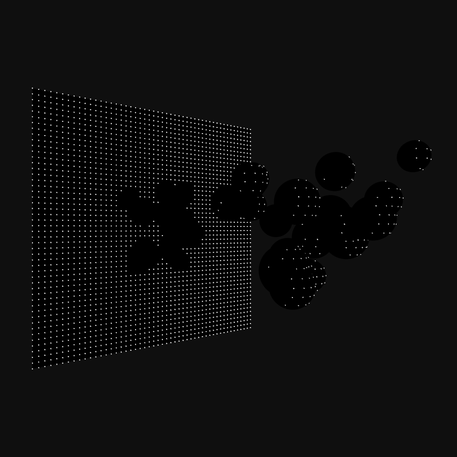
Since we can put the sphere wherever we want, we can add multiple spheres. Each particle is then tested against the different spheres one by one.
Distance Fields
In creative coding, it is often useful to have several perspectives to look at things. The equations above can be refactored:
\begin{cases} d( \vec{p} )-r<0, & \text{if } \vec{p}\text{ is inside} \\ d( \vec{p} )-r=0 , & \text{if } \vec{p}\text{ is on sphere}\\ d( \vec{p} )-r>0, & \text{if } \vec{p}\text{ is outside} \end{cases}
Nothing has really changed, the equations are still the same. But what they describe is a function {d( \vec{p} )-r} that separates space in three regions: one region outside the sphere, with positive values; one region inside the sphere, with negative values; and the surface of the sphere itself, where the function equals zero. This is the signed distance function of a sphere in the origin, with radius r .
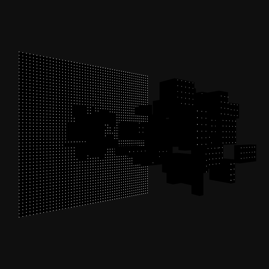
Testing the particles at each step is essentially the same evaluation: calculate the function at \vec{p} and see how it classifies. The advantage of seeing it this way is that the signed distance function can be easily replaced, and suddenly we’re checking collisions with a box, a torus, or any of the many shapes that have a well-defined sdf, like the list Inigo keeps.
In itself, there’s nothing stopping us from using the first approach to calculate the distance of a point to some specific geometry. But I find sdfs make it more intuitive, especially when we start modifying and combining them.
Not every function is a signed distance function, there are certain requirements. I’m not going into the rigorous math details, mainly because I’m not qualified enough to pull that off. In essence, its rate of change has to correspond to what you expect for a distance. If we follow the slope of the function downwards, we expect to end up at the surface. If we take small steps towards it, the distance should decrease with small steps, not suddenly change slope or start increasing.
As a creative coder, one of the first things we think of is “add noise”, which is not a mathematically valid distance function. Adding noise to the sdf of a sphere doesn’t give us the sdf of a noisy sphere. Fortunately, as creative coders, we can choose to forego the rigor and let the mayhem surprise us.
Tracer classes
Although a lot of information and functions are available online, it might not be immediately clear how to use any of it in Processing. Typically, code is given in OpenGL Shading Language (GLSL) and the used functions aren’t always obvious. GLSL is created to deal with numbers and vectors in a unified way. A function like max(v,0.0) looks familiar but in GLSL can also work component-wise on vectors, something that Processing doesn’t handle. Transcribing sdf functions can be confusing when unfamiliar with GLSL.
In this section, we’ll be creating the code used for the images above. In the end, we will have a rudimentary framework to build on for more complex pieces. Let’s start with some convenience classes, Point and Vector.
class Point {
  float x, y, z;
  Point(float x, float y, float z) {
    this.x=x;
    this.y=y;
    this.z=z;
  }
}
class Vector {
  float x, y, z;
  Vector(float x, float y, float z) {
    this.x=x;
    this.y=y;
    this.z=z;
  }
}
Both are just containers for coordinates. There is no real reason why we can’t use Processing PVector for this, or why we have both Point and Vector. But for this tutorial, it is easier to talk about points and vectors with as little abstraction as possible.
Another class that will come in handy is Ray, a half-line starting at a Point origin, the direction is given by the Vector direction. On creation, direction is normalized, its length is rescaled to 1.0. The function get(t) will return a new Point on the ray, a distance t from its origin.
class Ray {
  Point origin;
  Vector direction;

  Ray(Point origin, Vector direction) {
    this.origin=new Point(origin.x, origin.y, origin.z);
    float mag=direction.x*direction.x+direction.y*direction.y+direction.z*direction.z;
    assert(mag>0.000001);
    mag=1.0/sqrt(mag);
    this.direction=new Vector(direction.x*mag, direction.y*mag, direction.z*mag);
  }

  //Get point on ray at distance t from origin
  Point get(float t) {
    return new Point(origin.x+t*direction.x, origin.y+t*direction.y, origin.z+t*direction.z);
  }
}
For our mini-framework, we need signed distance functions. We could hardwire the functions into a sdf(Point p) function and change that code every time. But, a bit of structure goes a long way to help exploration. First, we need to tell Processing/JAVA what a signed distance function is:
//Interface that implements a signed distance function
interface SDF {
  float signedDistance(Point p);
}
Don’t worry if the details on what an interface is aren’t clear. We can consider it a promise to Processing: everything we identify as a SDF will have this function signedDistance(Point p) that returns a float. It doesn’t matter what class it is precisely, how we create objects of that class, how the object calculates the distance, as long as we tell Processing it’s an SDF, it will be able to call that function. An interface can be used to define variables, to pass objects to functions, pretty much everywhere we can use a class. What we can’t do, is create a new object with new SDF().
We already encountered one signed distance function, that of a sphere at the origin with radius r, {d( \vec{p} )-r}. We can now implement a class that encapsulates this.
/*
GLSL code https://iquilezles.org/www/articles/distfunctions/distfunctions.htm
float sdSphere( vec3 p, float s )
{
  return length(p)-s;
}
*/

class SphereSDF implements SDF {
  float radius;

  SphereSDF(float r) {
    radius=r;
  }

  float signedDistance(Point p) {
    return sqrt(sq(p.x)+sq(p.y)+sq(p.z))-radius;
  }
}
We tell Processing that this class implements SDF. In return, we need to fulfill our promise and implement signedDistance(Point p) . Everywhere Processing expects a SDF we can now pass a SphereSDF and it will work.
Similarly, we can define the sdf of a box at the origin of size X, Y, and Z.
/*
GLSL code https://iquilezles.org/www/articles/distfunctions/distfunctions.htm
float sdBox( vec3 p, vec3 b )
{
  vec3 q = abs(p) - b;
  return length(max(q,0.0)) + min(max(q.x,max(q.y,q.z)),0.0);
}
*/

class BoxSDF implements SDF {
  float X, Y, Z;

  BoxSDF(float x, float y, float z) {
    X=x;
    Y=y;
    Z=z;
  }

  float signedDistance(Point p) {
    float qx=abs(p.x)-X;
    float qy=abs(p.y)-Y;
    float qz=abs(p.z)-Z;
    return sqrt(sq(max(qx,0.0))+sq(max(qy,0.0))+sq(max(qz,0.0)))+min(max(qx, qy, qz), 0.0);
  }
}
One piece missing, the particles. We’re going to shoot particles, Tracers, into the scene along straight paths. When they hit something, they stop. Otherwise, they come to a stop after a certain distance. If our collision geometry would be defined by meshes, we could try to intersect the ray of the particles with the faces of the geometry. However, in this case, the whole point of this tutorial after all, we define the geometry by signed distance functions. So, we will be using another technique of finding collisions: sphere tracing.
Imagine we have an arbitrary collision geometry defined by a sdf and assume we have some particles starting outside this geometry. We know that in every point in space we can calculate the signed distance {sdf( \vec{p} )} . That distance, let’s call it d , tells us how close the geometry is to the point, but it doesn’t give us a direction. The only thing we can say is that the particle can safely move in any direction over a distance d . In other words, we know that at that point we can put a sphere of radius d and know for sure that the geometry isn’t in that sphere. In the extreme case, if the particle is moving straight towards the geometry, it might end up directly on the surface, but it will never cross it or go inside.
Take the figure below. We start at P_{0} and the chosen direction is along the blue line. The black triangle and rectangle are our collision geometry. sdf( P_{0}) tells us it that it is safe to move anywhere in the green circle centered on P_{0} .
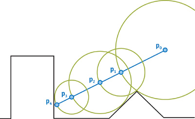
If we take a big step, the maximum safe distance, along the blue line, we end up in P_{1} . sdf( P_{1}) isn’t zero. Our direction of movement wasn’t the shortest path to the surface. We move on, this time a step of size sdf( P_{1}) and the particle ends up in P_{2} . We can repeat this until the returned distance is close to zero, or if we never hit the surface, after we reach a cutoff distance. In the figure, the fourth step takes us to P_{4} , on the surface.
The nice thing about this technique is that we don’t have to guess step sizes. There is no risk of taking too many small steps and wasting time, or of taking too large steps and overshoot a collision. The sdf automatically takes care of this by dynamically adapting the step size.
Our Tracer particle class looks like this:
class Tracer {
Ray ray;
float cutoff;
float precision;
float t;
float closestDistance;
int steps;
int MAXSTEPS=10000;
Point p;
Tracer(Point origin, Vector direction, float cutoff, float precision) {
ray=new Ray(origin, direction);
this.cutoff=cutoff;
this.precision=precision;
initialize();
}
void initialize(){
closestDistance= Float.POSITIVE_INFINITY;
t=0;
steps=0;
p=ray.get(0);
}
void trace(SDF sdf) {
p=null;
t=0.0;
steps=0;
do {
traceStep(sdf);
steps++;
} while (!onSurface() && tcutoff) t=cutoff;
p=ray.get(t);
}
void traceStep(SDF sdf){
float d=sdf.signedDistance(ray.get(t));
if (d
Each Tracer starts in a Point origin, along a Vector direction. Since our particles only move in a straight line, we store them as a Ray. We also need to define when we stop tracing the particles. Numerical roundoff makes it unlikely we'll get exactly 0.0 distance, so instead, we check if the distance becomes smaller than some value precison. If the tracer doesn't hit, we want to stop after a certain distance, called cutoff. Just to be safe, we limit the maximum number of steps our tracer can take, MAXSTEPS.
The current state of a Tracer is held in 4 variables:
t: the current distance traveled along rayclosestDistance: the closest the particle has come to the surface so farsteps: the number of steps taken so farp: the current position of the particle along the ray
At every step, the signed distance function is checked, and the particle is moved that distance forward along the ray. The tracing is stopped once one of three conditions is met:
closestDistance < precision: the particle has come closer to the surface than our precision threshold: collision.t>=cutoff: The distance traveled along the ray exceeds the cutoff distance: no collision.-
steps>=MAXSTEPS: The number of steps taken exceeds the maximum number allowed. This should only occur when we've made a mistake in the code.
In any case, at the end of the trace, the particle is either on the surface or beyond our region of interest.
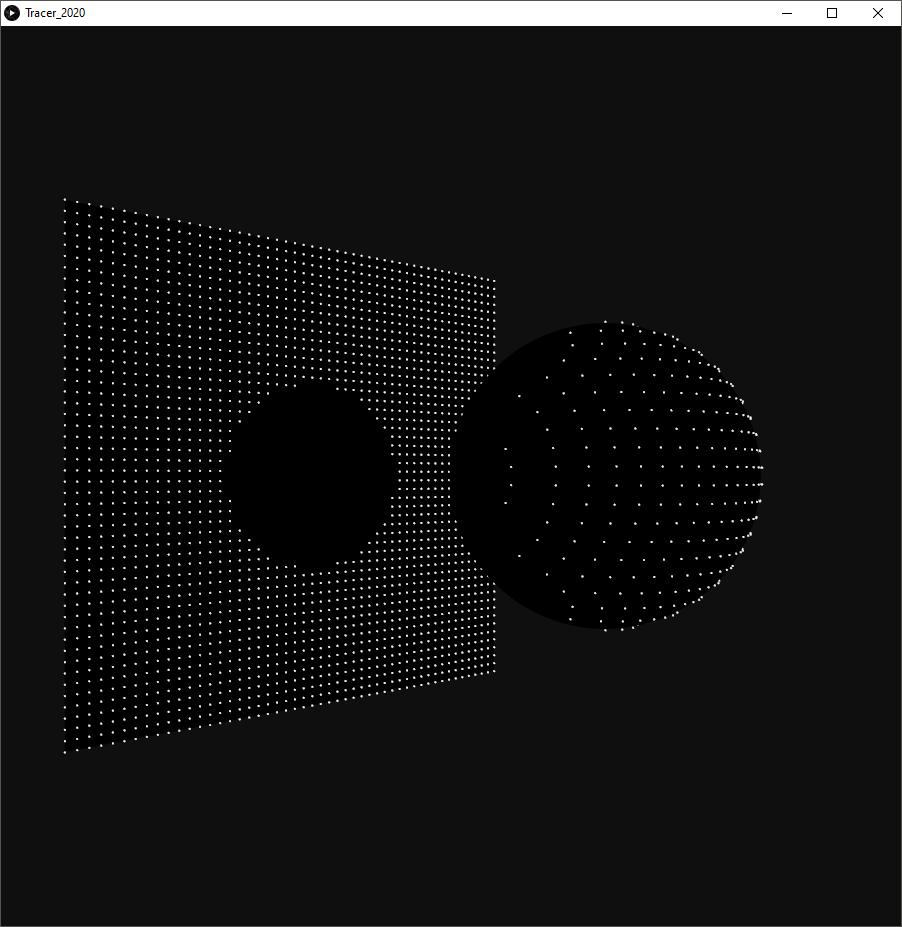
Putting it all together
To reproduce this image, we need to create a sdf, create some particles, and run the traces. The script, including the classes can be found here.
float emitterX, emitterY, emitterZ;
ArrayList tracers;
SDF sdf;
void setup() {
size(900, 900, P3D);
smooth(16);
noCursor();
createTracers();
createSDF();
trace();
}
void createTracers() {
tracers=new ArrayList();
float x, y;
emitterZ=500;
float cutoff=2*emitterZ;
int resX=50;
emitterX=600.0;
int resY=50;
emitterY=600.0;
for (int i=0; i
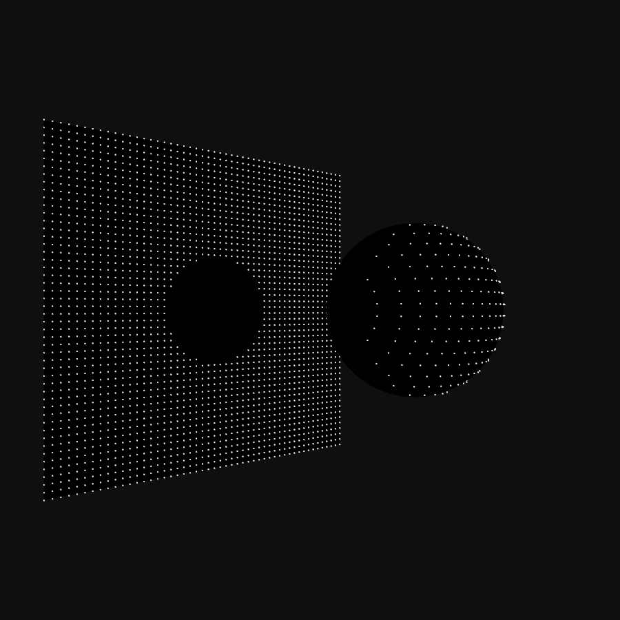
To setup the tracers, we create an emitter, a regular 600*600 square grid of 50x50 points. This emitter is positioned somewhere "above" the origin - to the right in the image above. Each point defines a Tracer aimed along the negative Z-axis. The sdf in this example is a single sphere at the origin. To show the tracers missing the sphere, we draw a limiting plane at the cutoff distance.
Beyond
This is just the start. In the next part, we will explore how we can extend the code to manipulate and combine signed distance functions.
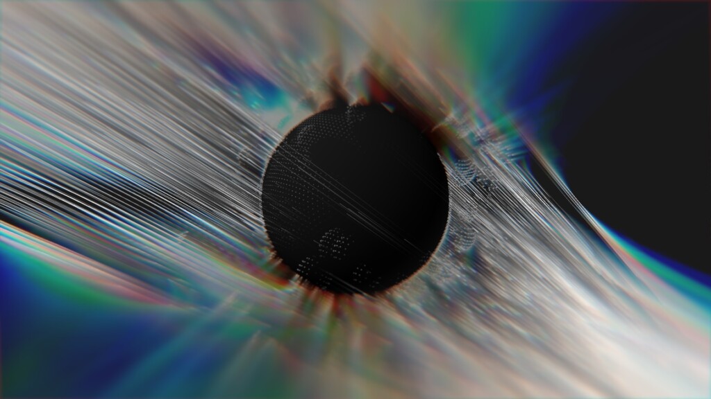
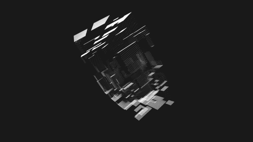
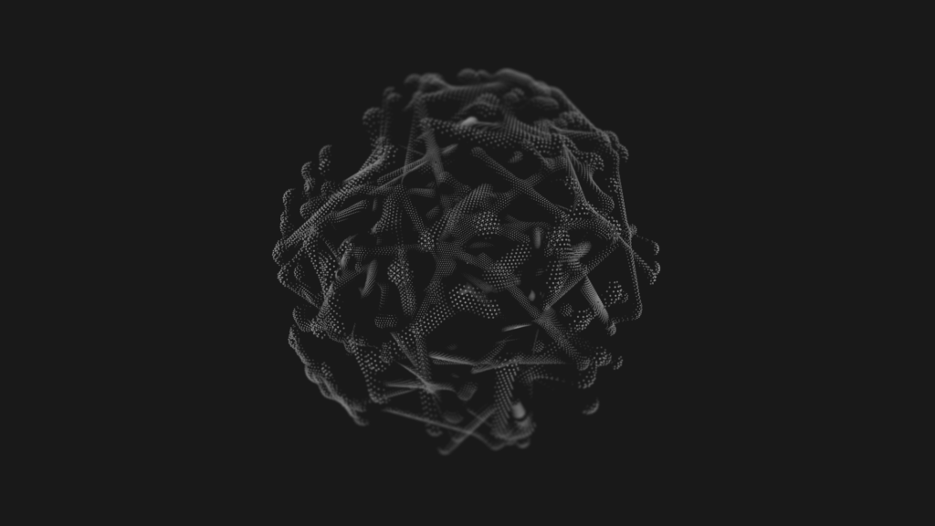
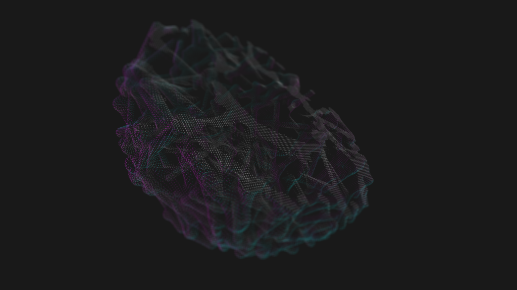
In 2017, I create a series of images using different combinations of tracers, sdfs and shader effects, that shows just some of the possibilities.